Histopathologic Cancer Detection

Relating to giving appropriate medical diagnosis, medical professionals are tasked with determining the validity and presence of any indicators that singal a disease. However, even among the best professionals, there is the possibility of human error. With image segmentation and classifier models becoming increasingly advanced through the years, the potential for them to aid in medical diagnosis by picking up potential misses by doctors appears more realistic.

utilizng the popular deep learning PyTorch library to classify microscope tissue images as either containing cancer or not. In addition to my own model, I'll show how the use of transfer learning can expedite model training and performance.

Code

The code is presented and documented in a jupyter notebook that provides step-by-step explainations.

Data

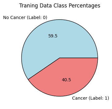
The dataset is available on Kaggle, and consists of 277,483 unique tissue images of lymph node cross sections. Imagse belong to one of two classes: no cancer, or cancer. Upon inspection, the dataset appears moderately balanced.

Below are a few randomly sampled images:

Preprocessing

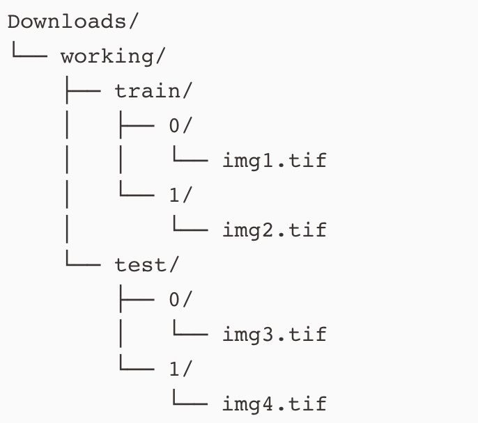
It is standard practice for supervised image-based tasks in machine learning to organize the images into a standard directory structure.

The reason for this is because when we call torch.utils.data.Dataloader on these images, the data loader will understand how to partitiion the data into batches for training.

To simplify and speed up training, 20,000 random images were sampled from the available 200,000, with stratification. This means that the class proportion shown above is preserved within these 20,000 samples.

Even when partitioning data randomly, it's best to be aware of the potential of bad sampling. For example, in the case that stratification was not employed, it is possible that we could have sampled a highly unbalanced proportion of images with the cancer label. This would lead to unnecessary complexity in model training.

If you have stronger hardware and resources, feel free to adjust the total number of samples for your model training. A test_size=0.3 was used. Label 0 coincides with no cancer, whereas lable 1 represents having cancer. After sampling with stratification and splitting the data into train and test sets, the results in the following:

Train Samples: 14,000

• label 0: 8,400
• label 1: 5,600

Test Samples: 6,000

• label 0: 3,600
• label 1: 2,400

Hardware

Training was performed on the CUDA platform from an RTX 3050 with 4 GB of VRAM.

Modeling

Both the simple and transfer learning model are based on utilizing a convolutional neural network (CNN) architecture. For my simple model, I implemented 2 convolutional blocks followed by a classifier layer. Each convolutional block consists of a sequential series of convolutions, pooling, and activation functions.

A concise explaination of CNNs can be found here.

When I first started learning about CNNs, the biggest challenge for me was understanding where the number of parameters of a model came from, and how the output's dimensions were determiined given an input of a certain dimension.

I understood the basic convolving process of sliding the kernel window and calculating the dot product. But where I find most online explainations lacking is detailing how the parameters passed in for the CNN code translate to what is happening conceptually. With a firm understanding of what part of a CNN that the code refers to helped expand my understanding of CNNs and neural networks in general.

The basic function for applying a convolution on a 2D image is nn.Conv2d(). I'll briefly explain the basic parameters to help elucidate what they mean for anyone learning about CNNs.

Basic Parameters:

• in_channels: the number of channels that the input into nn.Conv2d() has
  • channels refers to the layers of an input. In the instnace of an RGB image, it would have 3 channels, corresponding to the red, blue, green channel respectively. The shape of an image in tensor format can be represented in PyTorch as [channels, height, width].
  • Note that using matplotlib methods to display an image via plt.imshow() requires the channels to be the third dimension: [height, width, channels]. This can be accomplished using torch.permute()
• out_channels: the number of layers that the convolution output has
  • This is up to the scientist's choosing. If we input an RGB image into a convolution and specify the following parameters: nn.Conv2d(in_channels=3, out_channels=10), then the output will have dimensions [10, ? height, ? width]. The exact height and width are determined by the input's height and width along with the stride and kernel size used.
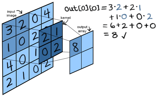
• kernel_size: refers to the height and width of the kernel filter. Below, we have a kernel of size 2, which specifies a 2x2 kernel.

A convolution calculation involves calculating the dot product between the overlaying kernel's values and the input's values. Then, we slide the kernel horizontally the number of pixels equal to the stride value. Then repeat the dot product. This continues until a new output (feature map) is created.

There is one kernel for each channel of the input. So an RGB image going through nn.Conv2d with out_channels = 10 has 3 x 10 = 30 kernels. The 3 kernels for 1 of the output channels have their results added together in the resulting feature map. Each output channel has its own bias terms. So in this case, there are 10 bias terms added to the output of each kernel's convolution respectively.

Simple Model

For baseline performance assessment, I implemented a simple deep neural network with 2 convolutional blocks. Each block includes a series of convolution, activtation function, convolution, acivation function, and ends with pooling.

The output channels after each convolution block was set to 10. After the second block, the tensor elements are flattened and connected to a fully connected layer of 1 neuron. 1 neuron was chosen because we are doing binary classification.

Transfer Learning Model

Transfer learning allows to speed up training because we can import a model with pre-trained weights. In this case, ResNet50 was chosen because it was trained on various images. What we change to make this model learn on our dataset is the fully connected layer. The steps are detailed below:

1. load pre-trained model
2. freeze all pre-trained weights
3. replace the model's fully connected layer with our own.

In our case of a binary classifier, we only need 1 neuron for our fully conencted layer, while maintaining the rest of the netowrk architecture.

During training, the weights between the flattened and our 1 neuron are what is being tuned to generalize on our dataset.

Results

Simple Model

Above we see that the baseline model performs relatively well from the start, better than a 50% accuracy by randomly guessing a sample's class. Training went for 30 epochs to observe the critical point of model overfitting. From the loss and accuracy plots, the training and testing loss diverge significantly around epoch 16. Thus future training can be early stopped here.

Another notable aspect of the plots are the spikes in decrease performance on the test set particularly in epoch 7, 12, 15. This could be due to encountering local minima in the loss function at these points when training on the training set. The model then adjusts in the next epoch, and we see test loss decrease close to the training loss as expected.

Furthermore, during data processing, transformations to the data include resizing to 64x64 and converting images to tensors for training. A seperate data transforming method includes augmentation such as horizontal flipping. Training was performed with and without this augmentation. The results displayed above are without augmentation for simplicity.

The loss and accuracy curves had a distictive feature such that train loss was always higher than test loss. Despite this, they both trended towards lower loss values over each epoch as the model better learned. Usually, we would expect the test loss to be higher than training loss because the model hasn't generalized to out of sample data in the early stages yet. However, I believe that the data augmentation transformation of horizontal flipping is one of the main reasons for observing a higher train loss throughout. That is because data augmentation introduces additional complexity that the model must learn, and makes it harder to generalize to such features. However, the test set is not augmented, and is simpler to predict on.

Transfer Learning Model

The loss curves from using the pre-trained resnet50 architecture shows that we are performing better than the simple model. The accuracy before overfitting in the simple model was around 82.5%, whereas the for the pre-trained model, we reach an optimal accuracy at the 7th epoch before overfitting at about 86%. Overall, we see that transfer learning allows for performance improvement, and in the case of a binary classification problem, we achieve results much better than 50% from randomly guessing.

Conclusion

Overall, we demonstrated how to build a neural network and implement methods to train and evaluate our models using PyTorch. In addition, we observe the benefits of utilizing transfer learning to speed up the training process and increase model performance.

Although an optimal 86% accuracy on the transfer learning model is nice for demonstration purposes, if the scaling of such models for serious real life medical applications in detecting cancer, then we would like this metric to be much closer to 100% correct as possible.

As models continue to improve, it's also important to understand that currently they are more of an aid, than a total replacement for medical professionals. Human error occurs, and these models can help mitigate this by allowing us to analyze the discrepencies between the human and model's predictions.